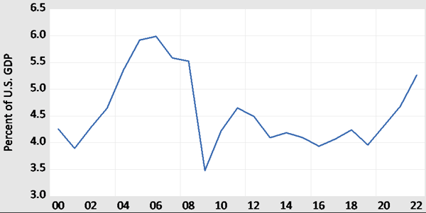
The U.S. current account deficit has increased from 2.1% of GDP in 2019 to 3.7% of GDP in 2020 to 4.8% of GDP in the first quarter of 2022. The Bureau of Economic Analysis reported that this increase is driven by a growing deficit in goods trade. Figure 1 plots the U.S trade deficit in goods.

Recent trade and current account deficits emerged in the context of large U.S. budget deficits, rising interest rates in the U.S. relative to its trading partners, and an appreciating U.S. dollar. In the 1980s the U.S. also had large budget deficits, higher interest rates relative to its trading partners, and an appreciating dollar. In the 1980s the strong dollar caused U.S. exporting and import-competing firms to lose price competitiveness. In 1985 the U.S. ran trade and current account deficits of 3% of GDP.
The G-5 countries (France, Germany, Japan, the UK, and the U.S.) were alarmed by these imbalances. To resolve them they reached the Plaza Accord in September 1985. The U.S. agreed to reduce its budget deficit, America’s trading partners implemented stimulative policies, the five countries worked together to reduce the value of the dollar, and all agreed to fight protectionism. The dollar did depreciate and the U.S. current account reached balance in 1991.
Estimating Trade Elasticities
Exchange rate adjustments seemed to help rebalance trade after the Plaza Accord. To investigate whether they would have this effect now I estimate U.S. import and export elasticities. In previous work, Chinn used dynamic ordinary least squares (DOLS) techniques to estimate trade elasticities for U.S. imports and exports over the 1975Q1-2010Q1 period. In his baseline specification, he reported an exchange rate elasticity of -0.45 and an income elasticity of 2.6 for goods imports excluding oil. For goods exports excluding agriculture he found an exchange rate elasticity of 0.6 and an income elasticity of 1.9.
I estimate aggregate import and export elasticities using data on goods imports excluding oil and goods exports from the U.S. Census Bureau and the U.S. International Trade Commission. These are deflated using import and export price data obtained from the U.S. Bureau of Labor Statistics. Following the imperfect substitutes model, imports are assumed to depend on the real exchange rate and GDP in the U.S. and exports on the real exchange rate and GDP in the rest of the world. Data on the broad consumer price index deflated real effective exchange rate are obtained from the Bank for International Settlements and data on U.S. GDP from the OECD. Data on GDP in the rest of the world are calculated as a geometrically weighted average of GDP in 15 leading trading partners, where the GDP data come again from the OECD. The model is estimated using DOLS and data extending from 1994Q1 to 2019Q4. Four lags and two leads of the first differenced right-hand side variables, quarterly dummies, a time trend, and dummies for the Global Financial Crisis are also included in the model.
The resulting import function is:

In equation (1) IM represents U.S. real imports excluding oil, RER represents the real effective exchange rate, and USGDP represents U.S. real GDP. The results indicate that a 10 percent dollar appreciation would increase imports by 5.0% and that a 10% increase in U.S. GDP would increase imports by 21.0%.
The corresponding results for exports are:

In equation (2) EX represents U.S. real exports, RER represents the real effective exchange rate, and ROWGDP represents real GDP in the rest of the world. The results indicate that a 10 percent dollar appreciation would reduce exports by 5.2% and that a 10% increase in rest of the world GDP would increase exports by 31.7%.
Implications
The Marshall–Lerner condition states that, beginning from balanced trade, a currency depreciation will improve a country’s trade balance if the sum of the absolute values of the export and import elasticities exceeds one. The price elasticities in equations (1) and (2) just meet this condition. This suggests that a dollar depreciation would help to improve the trade balance
Between 2000 and 2021, the U.S. current account deficit averaged 3.4% of U.S. GDP. So far the rest of the world has been willing to finance these U.S. deficits. If the rest of the world grows unwilling to continue accumulating U.S. assets on this scale, the dollar will depreciate. The results above indicate that the depreciation will help to improve the trade balance. However, the price elasticities are not large. This implies that a depreciation alone will not be enough to rebalance trade. This would force some of the adjustment to come through a fall in U.S. GDP. Such an adjustment would prove painful for U.S. workers, consumers, and firms.
The U.S. budget deficit has averaged 6.6% of GDP over the last 12 years. This fiscal stimulus increases U.S. GDP and thus the U.S. current account deficit. The U.S budget deficit that caused consternation in 1985 was below 5% of GDP. So the U.S. budget and current account deficits that led to urgent action in the Plaza Accord are now exceeded year after year. Both to help reduce the current account deficit and to help fight inflation, the U.S. should reduce its budget deficit.
This article first appeared on Econbrowser on September 15, 2022. Reproduced with permission.


